Most folks would agree that men tend to be more aggressive than women. We observe this in other mammals too. Quantifying the difference, however, presents a problem. The variable, 'aggressiveness,' is fuzzy. It is not like height or weight. We have no rulers or scales for it. Nevertheless, group differences in fuzzy variables can be precisely determined. For this purpose, we introduce the method of thresholds, and illustrate its use by assessing the aggressiveness gender difference.

Aggressiveness by Gender
   Like other fuzzy variables, aggressiveness exhibits a range of values. In fuzzy language we might say it varies from timidity to extreme aggression. We could find ways to express intermediate values, but the fuzziness of language will limit exposing all the shades and nuances of the property. The method of thresholds sidesteps this limitation. It requires only a smidgen of data. First, we identify one non-fuzzy point on the variable's value spectrum -- a threshold point. For aggressiveness, we choose the threshold to be the point where aggression leads to assault. Additionally, we need to know the proportions of each group that reach or surpass the threshold.

   Several data sources list the proportions of men and women who commit assault in any given year. The best of these is the National Crime Victimization Survey (NCVS) of the Justice Department. Each year it canvasses a representative sample of about 80,000 Americans, from roughly 43,000 households. From the responses, a picture of crime emerges that does not depend on apprehending criminals or even reporting crimes. The last full report of the NCVS, issued in 1994, lists the number of single-victim assaults in the nation for that year, and the perceived sex of the offenders. 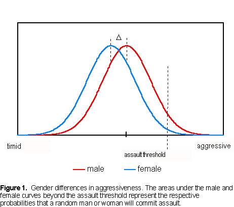From these data and population estimates from the Census Bureau, we discover that 0.961 percent of women and 4.51 percent of men perpetrated some kind of assault in the U.S. in 1994.

   Figure 1 shows male and female distributions for aggressiveness. We assume them to be normal. The assault threshold shown in the figure has been placed to make the area to its right and under the male (red) distribution 4.51 percent of the total. The female (blue) distribution has been displaced to make the area under it and to the right of the assault threshold 0.961 percent of the total. When these conditions are fulfilled, the resulting 'distance,' Δ, between the two distributions is the mean gender difference for aggressiveness in standard deviation units (SD). A procedure for doing this analytically is presented in Appendix A. Note, we neither defined the fuzzy variable nor created a scale for measuring it to obtain its group difference. Using NCVS data in this way, the male - female mean difference, Δ, is 0.65 SD. That is, men are more aggressive than women by 0.65 SD.

   Most Hispanic Americans classify themselves as white. If victims are given a binary choice, they too will usually describe Hispanic assailants as white. That aside, we find from NCVS and census data that 2.20 percent of whites and 5.00 percent of blacks were perceived as assailants in 1994. Again, using assault as a threshold for aggressiveness, the method of thresholds finds that whites are less aggressive than blacks by 0.37 SD.

   To include Asians in our study, we turn to data gleaned from INTERPOL year books by J. Philippe Rushton (Society, Jan-Feb 1995). Rushton looked at 23 predominantly African countries, 41 Caucasian, and 12 Asian countries. Per 100,000 members of each group, he found 'serious assault' rates of 213, 63, and 27, respectively. Applied to these numbers, the method of thresholds yields a black - white mean difference for aggressiveness of 0.37 SD in perfect (if fortuitous) agreement with NCVS assault results, this despite that the INTERPOL threshold for serious assault is much higher than the NCVS standard. The white - Asian mean difference from these data is 0.24 SD. Of the three groups, Asians are the least aggressive, blacks the most. The 'distance' between blacks and whites is about 50 percent greater than between whites and Asians. Table 1 summarizes the results as Standard Aggressiveness Values.

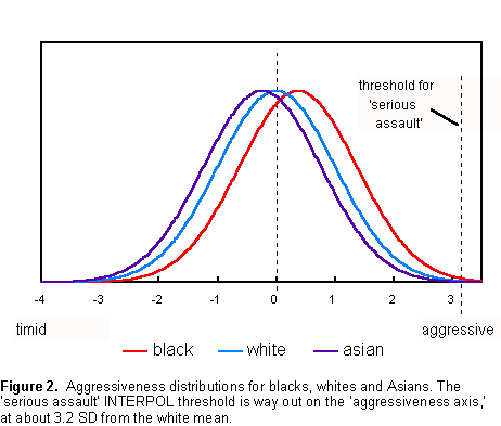
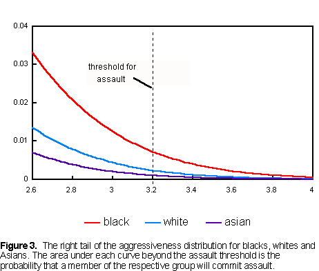
   Figure 2 presents the aggressiveness distributions for blacks, whites and Asians determined from the INTERPOL data. From them we see that the threshold for 'serious assault' is way out on all three curves (3.2 SD from the white mean). On this scale, most people in each of the three races will tend to be neither particularly timid nor aggressive. They mostly fall within one standard deviation of the white mean.

   Figure 3 zooms in on the region of extreme aggressiveness. The areas under the curves beyond 3.2 SD represent the respective probabilities that a random black, white or Asian will be aggressive enough to commit assault. In the right tail, aggressiveness probabilities are small, but they show that compared to whites and Asians, blacks are much more likely to be extremely aggressive.

   Using Department of Justice data, we constructed a scale of Standard Criminality. On it we placed black males, blacks, Hispanic males, Hispanics, white males, whites, black females, Hispanic females and white females. As a non-fuzzy threshold for criminality we chose incarceration rate. Incarceration meets all our requirements. It is non-fuzzy, unambiguously related to criminality, and reliable data are available. The Department of Justice publication, Prisoners in 1998, lists incarceration rates for 1997. Most notably, it breaks out Hispanics from non-Hispanic whites and non-Hispanic blacks. Some data from this publication are reproduced in Table 2 along with quantities derived from them.

   From the incarceration rates in Table 2, using the method of thresholds, we constructed a table of Standard Criminalities (Table 3).

   We also investigated how mean differences in criminality vary with time. Time invariance would suggest that criminality is an inherent property of a group. Unfortunately, time series data from the Justice Department does not split out Hispanics from whites and blacks. Though corrupted in this way, these data can still be used to answer the time invariance question. In the decade spanning 1987 to 1997, incarceration rates almost doubled, but group criminality differences remained almost constant. Including Hispanics, the mean criminality differences between white and black males for the years 1987, 1992 and 1997 were 0.842 SD, 0.852 SD and 0.842 SD, respectively.

   Finally, if standard criminalities are characteristic of groups, they should also remain invariant across international boundaries. We looked at incarceration rates from the U.K. reported by the Home Office in its publication, Prison Statistics England and Wales 1995. According to the Home Office, 134 whites and 1049 blacks per 100,000 of each group were imprisoned. The method of thresholds crunched the U.K. data to yield a black-white mean criminality difference of 0.694 SD. This may be compared with the black-white difference of 0.736 SD for American blacks computed from standard criminalities in Table 3. The results strongly suggest the inherent character of criminality. Though U.S. incarceration rates for each group are significantly greater than those in the U.K., the black/white criminality differences are within 0.04 SD of each other. We have observed analogous occurrences in seemingly unrelated spheres. Math SAT scores, for example, increase linearly with family income for both blacks and whites, but the racial gap remains constant at about 1 SD.

Sex Drive by Race and Hispanic Origin
   The method of thresholds requires a well defined, measurable point on the sex-drive scale. Venereal disease rates provide such a point. You get gonorrhea by being promiscuous, and sex drive leads to promiscuity. Like incarceration, gonorrhea is a yes/no proposition. Either you have it or you don't. We consulted Arthur Hu's Index of Diversity for rates of gonorrhea by race and Hispanic origin. (If you have not visited Hu's page, you should. It is a virtual encyclopedia of ethnic and racial Information.) Hu's data, taken from a CDC source, are presented in Table 4.

Games with Fuzzy Variables
   Standard values for fuzzy variables are not just another way to express race, gender and ethnic differences. They arm us with predictive and analytical power. As an example, consider an issue that receives considerable attention in the popular media, and sometimes in the courts - the disproportionate suspension of black high-school students. Addressing this issue, we ask the following question:

Suppose a half-white, half-black school system suspends 1 percent of its students for disruptive behavior. What is the most probable racial makeup of the suspended group?

###

APPENDIX A. Standard Values of Fuzzy Variables.

   Let P(x) be the normalized probability distribution of some fuzzy variable, x, for some reference group, say Group A. Let Δ be the mean difference (in standard units) between the function, P(x), and the corresponding distribution of the same variable, P_B(x), for Group B. The distribution functions for the two groups are assumed related by the translation, P_B(x) = P(x-Δ). The quantity, Δ, is the standard value of the fuzzy variable for Group B.

   Let f be the fraction of the reference group reaching or surpassing some threshold value, λ, of the fuzzy variable. The quantities, λ and f are related as follows:

   Knowing the fraction, f, (A.1) may be used to obtain a value for the threshold, λ, in standard units. With this threshold in hand and the value of f_B , (A.2) yields Δ, the standard value of x. The tables of standard values found in the body of this essay were produced in this way, taking P to be Gaussian,

APPENDIX B. Games

   The suspended-students problem can be solved by viewing it as one in which slots are filled in rank order of aggressiveness. The number of slots is the number of suspended students. Essentially, we find the most aggressive student and throw him into one of the slots. Then we throw the next most aggressive student into a vacant slot, continuing until all slots are filled.

   In general, suppose N_S slots are to be filled in rank order on some property from a pool made up of N₁ members of Group 1, N₂ members of Group 2, etc. Members of all groups will be selected to fill a slot if they have a property value equal to or greater than some threshold, . The threshold, λ, is the value of the property exhibited by the last person to fill a slot. It is determined by the pool sizes, the number of slots available and the property distributions for each group. The variables are related as follows:

where P_i is the normalized distribution function of the property for group i.

   We have assumed previously that P_i (x) = P(x - Δ_i), where P is the distribution for a group designated as the reference group. Accordingly, Equation B.1 may be written as:

   Each term on the left side of (B.2) represents the number of members from the corresponding group who fill slots. The terms sum to the number of slots, N_S. From the pool sizes (the N 's) the number of slots, N_S, and the standard values of the property (the Δ's), we find the threshold value, Δ, by solving (B.2) numerically. The standard value (Δ) for the reference group is zero. Knowledge of it allows evaluation of each term, giving the number selected from each group.

   Another form of (B.2) is convenient for processing data given as percentages of a population. The high-school student suspension data were given in this form. Multiplying (B.2) thru by 100/ΣN_i gives