Complete contents of La Griffe
Write La Griffe

 

INTELLIGENCE, GENDER AND RACE:

CONVERSATION WITH A PRODIGY

General intelligence, its form and how it is distributed in various populations are among the topics covered in this conversation with Prodigy. A new kind of meta-analysis is unveiled, and with it an assessment of the cognitive gender gap. All this and more when La Griffe du Lion interviews a celebrated whiz kid.

"If he wished, one could make an IQ distribution look like the distribution of molecular speeds."

-- Prodigy, 2006
On the arbitrariness of IQ

La Griffe du Lion: I understand this is the first interview you've granted. To what do we owe this privilege?

Prodigy: Actually, no one ever asked me.

LG: Well, we are nevertheless honored. Here at La Griffe du Lion we think it quite remarkable for someone so young to have solved so many problems. How have you found the time?

P: The secret is to utilize those times of day taken up with mindless but necessary activity. For example, I developed Smart Fraction Theory while brushing my teeth.

LG: What you've been up to lately?

P: A few months ago I came across a paper by D. N. Jackson and J. P. Rushton (Intelligence 34 (2006) 479-486), in which they reported that men had a 3.63 IQ-point advantage over women.

LG: I recall the paper well. It caused quite a media stir.

P: That's correct. Professor Rushton even made several TV appearances. After seeing him on the Paula Zahn show it occurred to me that I could capture some of the media spotlight for myself by conducting my own investigation of cognitive sex differences.

LG: I must warn you there can be consequences to going public on matters of group differences. Psychologist Helmuth Nyborg recently lost his job after he published a study showing a male cognitive advantage.

P: Not to worry. I don't have a job.

LG: Tell us then what your investigation revealed?

P: Actually, my most important finding is not directly concerned with gender issues. It is more ecumenical in scope.

LG: Oh?

P: Yes, I had a particularly large laundry to do.

LG: Laundry?

P:  Yes, I began my search for a cognitive gender gap while waiting for my laundry to dry. The load was sufficiently large that I had time not only to characterize the gap but also to demonstrate this important proposition:

A single, Gaussian-distributed variable uniquely determines the dense rank order of performance on large-scale standardized exams. The variable completely accounts for group differences in test performance.

LG: Sounds a lot like g, the general mental-ability factor.

P: It does.

LG: But you claim that g is Gaussian-distributed. In The g Factor, Arthur Jensen asserts that the form of the population distribution of g is not known, and presently there is no way to determine it. Do you disagree with that?

P: The form of the g distribution is not known directly, but just as the lion is known by his claw, so the form of the distribution can be inferred from its consequences. Much of what we know about nature has been acquired in this way. The existence of dark matter, for example, is inferred from its gravitational effects on visible matter. Similarly, by examining the observable consequences of a Gaussian g distribution we can confirm its existence. We simply need to know what to look for and where to look for it.

Quite apart from experiment, there are good theoretical reasons to expect the distribution of g to be Gaussian. To the extent that an individual's intelligence is the result of many additive factors, both genetic and environmental, the central limit theorem assures that its distribution will be approximately Gaussian in large populations. Moreover, mental ability in populations of test takers results from the same additive factors that determine intelligence in the general population. Consequently, we might expect to find Gaussian distributions of g not only in the general population, but also in the more circumscribed population of test takers. Typically, high-stakes standardized-test samples are large, often numbering many thousands. For our purposes, that more than satisfies any sample-size requirement imposed by the central limit theorem. Do you think Paula Zahn might be interested in the central limit theorem?

LG: I'll make some inquiries. But meanwhile tell us if the central limit theorem implies that IQ distributions should be Gaussian as well?

P: No, IQ distributions are approximately Gaussian but that has nothing to do with the central limit theorem. IQ raw scores are massaged with a transformation, forcing their distribution to look Gaussian. But that is just a mathematical trick. The distribution of IQ could just as easily be made to look like the Maxwell-Boltzmann distribution of molecular speeds. On the other hand, the Gaussian distribution of g is the work of Nature.

LG: If the form of the IQ distribution is arbitrary, what value are IQ tests?

P: They serve the important function of ranking people according to mental ability. If, for example, A, B and C have IQs of 80, 100 and 120, respectively, we can say that C is more intelligent than B, who in turn is smarter than A. But we cannot say that C is smarter than B by the same amount that B is smarter than A.

LG: What else have you found.

P: I developed  powerful new analytical tools and with them reassessed the cognitive gap between African Americans and Non-Hispanic whites.

LG: But that is among the most studied of all group differences. Why would you want to reexamine it?

P: Precisely because this gap has been so well-studied; what better way to test a new analytical procedure? Here is the result of my analysis:

A white-black mean difference in g of 1.09 SD exists in favor of whites, equivalent to 16 IQ points. The black g distribution is narrower than the white, with a variance ratio (B/W) of 0.888.

As you see there are no surprises.

My principal goal, however, was not to elucidate the well-known black-white gap but rather to determine the male-female difference in general intelligence. Studies have yielded a large spread of results running from no gap at all to more than 8 IQ points in favor of men. Here is the result of my analysis:

A male-female mean difference in g of 0.162 SD exists in favor of men, equivalent to 2.43 IQ points. The female g distribution is narrower than the male, with a variance ratio (F/M) of 0.916.

You will find these to be the definitive estimates of both the white-black and male-female cognitive gaps. They follow from the most elegant analysis of the largest samples ever examined.

LG: Had you not better tell us how you obtained these results so La Griffe's readers can determine that for themselves.

P: In truth I think Geraldo would be a better venue for me to reveal the details of the methodology. He has a much larger audience than La Griffe du Lion.

LG: Yes, but like its host Geraldo's audience is largely innumerate. La Griffe du Lion can guarantee you a smaller but more select audience said to be the quintessence of perspicacity and refinement.

P:  OK, I am convinced. Suppose I provide you with a general outline, and include additional details in an Appendix for your readers to examine at their leisure.

LG: Do it!

Diversity space
P: Let me introduce you to diversity space. It is a construct I find convenient for comparing group mental abilities. Each point in diversity space specifies the proportions of two groups that attain some threshold of cognitive achievement. Look at Figure 1. There, the point (0.6, 0.4) is represented in the diversity space of Groups A and B. It corresponds to 60% of Group A and 40% of Group B reaching some unspecified threshold of cognitive achievement.

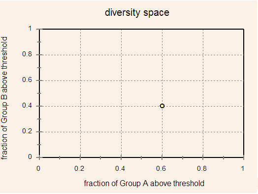
Figure 1. The point (0.6, 0.4) in diversity space corresponds to a cognitive threshold of achievement reached by 60% of Group A and 40% of Group B.

In diversity space, specific thresholds of achievement are not specified. The point (0.6, 0.4) could arise from any mental challenge met by 60% of Group A and 40% of Group B. Such a challenge might, for example, be passing the bar exam or reaching 1200 on the SAT. The possibilities are countless, the details not important. Points in diversity space are not test specific. They are ability specific.

The locus of points in diversity space
P: Only certain points in diversity space are allowed. Their locus is uniquely determined by the group distributions of g. Figure 2 shows the locus of points for two groups with identical g distributions. It is a line of unit slope through the origin, reflecting the fact that all cognitive thresholds will be reached by equal proportions of the two groups.

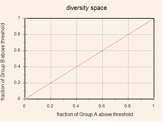
Figure 2. The locus of points in diversity space for two groups with identical distributions of g.

In general, however, g distributions will vary by race, ethnicity and gender. If the g distributions are known for two groups, we can find the locus of allowed points in their diversity space. Figure 3 displays an assortment of loci generated from Gaussian g distributions for Groups A and B. The curves differ from one another only in the choice of parameter values. To generate them, nothing whatsoever was assumed about test-score distributions.

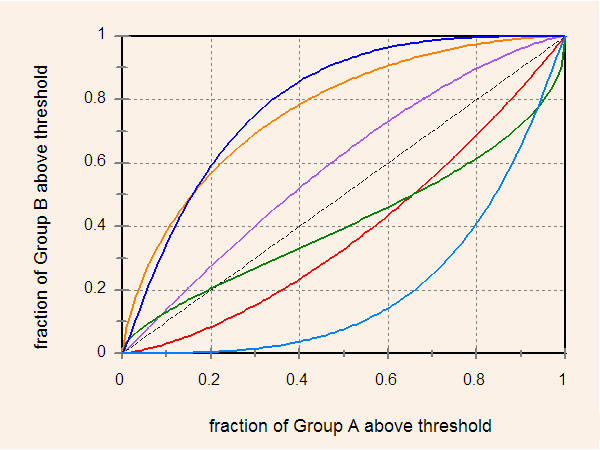
Figure 3. Loci of points in diversity space for Gaussian distributions of g. The curves differ from one another in the choice of parameter values.

LG: Could you spell out more about how the curves in Figure 3 were generated?

P: Here's the short version. (I'll provide a bit more detail in the Appendix.) Let P_A be the probability density function of the g distribution in Group A, and f_A the fraction of group A that succeeds in performing some cognitive task. The minimum value of g, say Λ, needed to succeed is given implicitly by the relation:

with a similar relation for Group B:

The pair of equations (1) and (2) taken together relate f_B to f_A parametrically. The curves in Figure 3 were generated for P_A and P_B Gaussian.

The elevation of meta-analysis
I now assert that a single Gaussian-distributed latent variable, plausibly g, uniquely determines the dense rank order of performance on large-scale standardized exams. There is a simple test of this proposition. If it is true, there will exist a single curve, derived from Gaussian distributions of g, upon which all observed points in diversity space, irrespective of their source, must lie. We merely have to find that curve.

Consider first the diversity space of blacks and Non-Hispanic whites. Seven points, chosen to span the range of proportions in diversity space, were obtained from five different large-scale standardized tests. Here is a brief description of the tests and sample sizes when available.

SAT: Composite scores (V+M) from the 2000 administration taken by 119,394 blacks and 717,632 whites.

CBEST: (California Commission on Teacher Credentialing) 2000-04 first-try pass rates of 15,466 blacks and 160,393 whites.

MCAT: 1993-95; taken by 8,698 blacks and 74,213 whites.

Bar exam: Data from 1) NY bar exam 1985 through 1988; first-try pass rates (sample sizes were unavailable, but typically run more than 7,000 per test administration), and 2) all US law students beginning law school in fall 1991; first-try pass rates of 1,368 blacks and 19,285 whites.

ACT: 2006; fractions meeting all 4 ACT College Readiness Benchmark Scores; taken by 139,118 blacks and 760,084 whites.

Using the least squares criterion parameters of the g distributions were adjusted to obtain the best fit. Figure 4 shows the result.

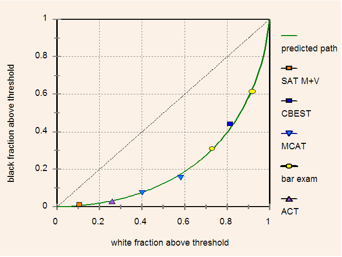
Figure 4. Seven points in white-black diversity space obtained from five separate standardized tests. The theoretical locus of points is shown as a solid green curve.

Although the observed points in diversity space were obtained from five different standardized tests they all lie close to the theoretical curve predicted by Gaussian distributions of g for both whites and blacks. Adjusted parameter values yielded a mean white-black difference of 1.09 SD equivalent to 16 IQ points in favor of whites and a variance ratio (B/W) of 0.888.

LG: Impressive fit! I presume you looked next for a gender gap.

P: That's correct. After all, it was the search for a cognitive gender gap that prompted this inquiry.

MCAT data were not available disaggregated by sex, so I substituted (1989-1990) LSAT data in their place. Sample sizes were generous: CBEST 89,110 men, 188,975 women; Bar exam 13,872 men, 10,937 women; SAT 574,715 men, 673,620 women; ACT 517,563 men, 646,688 women; and LSAT 67,968 men and 52,734 women.

Figure 5 shows 15 points in diversity space obtained from these five standardized tests. Again, all observed points fit closely to the theoretical curve predicted by Gaussian distributions of g in both men and women.

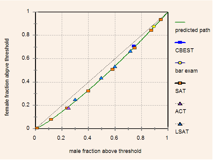
Figure 5. Points in male-female diversity space obtained from five different standardized tests. The theoretical locus of points is shown as a solid green curve.

Parameter values adjusted to the best least-squares fit yielded a male-female g gap of 0.162 SD equivalent to 2.43 IQ points in favor of men, and a variance ratio (F/M) of 0.916. Figure 6 compares the two g distributions on the same axes.

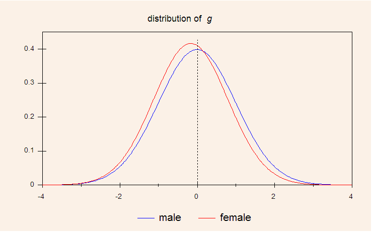
Figure 6. The distribution of g in male and female populations. The scale of the abscissa is in units of the male standard deviation.

LG: It seems that there is an insignificant difference separating men and women.

P: That depends on the context.

LG:  Wouldn't you call a difference of less than 2.5 IQ points small?

P: Again, that depends on the context. For example, suppose we ask what the chances are that a randomly selected woman is smarter than a randomly selected man. Based on their g distributions, I calculate that the woman has better than a 45 percent chance of being smarter than the man.

LG: I'd say that difference is barely noticeable.

P: I agree. Based on this criterion male-female cognitive differences would mostly go unnoticed

LG: What other criteria are there?

P: The marketplace provides good examples. Linda Gottfredson has studied cognitive demands of various occupations. In her paper, Why g Matters (Intelligence, 24(1), 79–132) she estimates a minimum IQ of 120 is needed to be competitive in moderately "high-level" jobs such as research analyst or advertising manager. A gender gap of 0.162 SD with a variance ratio 0.916 tells us that of the workforce segment meeting this requirement only 37% will be female. The g distributions will impose not a glass but rather a statistical ceiling on women in the high end of the workforce. According to EEOC, in 2003, 35.2% of "officials and managers" in the private sector were women -- a number suspiciously close to 37%. Interestingly, among federal employees women held 66% of the "management" jobs. But that is the stuff of another investigation.

LG: Thank you Prodigy, I've enjoyed our conversation immensely. I do appreciate your gracious acceptance of my invitation and hope that as a result you don't suffer unwarranted disapprobation.

P: Again, not to worry. In the worst-case scenario I could apologize, attribute my transgressions to alcohol, and raise funds for Rainbow/Push and NOW. I might even meet some beautiful addict in rehab. For now, however, I have a big load of laundry to do.

###

APPENDIX


A few details

Given that the distribution of g converges to normality in large populations, the g-distribution probability density function will be approximated by:

where μ and σ are the mean and standard deviation, respectively. We choose for convenience the unit of g to be one standard deviation of the Group A distribution. Also, since g has no absolute zero, we are free to set it as we wish. Accordingly, we choose the zero of g to be its mean value in Group A.

With these simplifications the fraction of Group A that reaches or exceeds some cognitive threshold, Λ, is:

with a similar expression for the corresponding fraction of Group B:

In (A.2) and (A.3), Δ is the mean g difference (A - B) between Groups A and B, and ρ is the dimensionless ratio of standard deviations, σ_B/σ_A.

Equations (A.2) and (A.3) relate f_A and f_B parametrically. For a given value of f_A, Λ may be obtained numerically from (A.2). This value in (A.3) returns the fraction f_B. The curves in Figure 3 were generated in this way for various values of ρ and Δ. For the analysis of data, whites and males correspond to Group A, blacks and females to Group B. Values of f_B calculated from (A.3) were fit to observed values by adjusting the parameters Δ and ρ to satisfy the least squares criterion.

Who's smarter, Random Man or Random Woman?
The probability that Random Man's general intelligence, g, lies between y and y + dy is P(y, 0, 1)dy. Let f(y) be the probability that Random Woman's general intelligence, g, is greater than y. That is,

The conditional probability that Random Woman is smarter given that Random Man's g is between y and y + dy is f(y)P(y, 0, 1)dy. Integration over all values of y gives the probability, p, that the woman is smarter, i.e.,

Using the least squares values for Δ and ρ, (A.5) returns 0.453 for the probability that the woman is smarter.

###