April 2006
Complete
contents of La Griffe
Write La Griffe
POLITICS, IMPRISONMENT AND RACE
An adult black man is seven times more likely than his white counterpart to reside behind bars. Paradoxically, the largest disparities are found in political domains controlled by liberals -- the leaders in the struggle for racial justice. By examining how criminal behavior is distributed within the races, the paradox is resolved showing it to be an unintended consequence of liberal benevolence and goodwill.
"One should not increase, beyond what is necessary, the number of entities required to explain anything."-- William of Ockham (1285-1349)
Prodigy's
Sociology Colloquium lecture, April 2006
It was uncommonly kind of Uncle Steve to invite me here this afternoon to participate in your Sociology colloquium Series. I am delighted to be here, to meet so many of you, and to join more of you later for dinner.
Skimming through the titles of past colloquia, I found that certain words or their cognates occurred with conspicuous frequency, among them: race, politics and prison. My lecture today concerns each of them -- more specifically their relationship to one another.We all know that African Americans are imprisoned disproportionately to their numbers in the general population. According to the last decennial census a black man was 7.4 times more likely than his white counterpart to be incarcerated. In the language I'll use today, we would say that the disparity or incarceration ratio was 7.4. State-by-state, the figures varied widely from 3.1 to 29.3. But contrary to expectation, the highest disparity ratios turned up mostly in politically progressive states, while the smallest ratios were mostly found in conservative states. Though the numbers change a bit from year to year, this racial-political pattern of imprisonment endures. One of the questions I will answer today is, why?
Many here have devoted their professional lives to eliminating racial disparities in prison and of course elsewhere. And most of the rest of us are philosophical allies sympathetic to this ideal. Consequently, it must be disconcerting to find the greatest black-to-white imprisonment ratios in your own ideological backyards. But be assured this is not the result of unconscious, repressed racism, but rather the innocent product of your goodwill -- an accidental consequence of liberal philosophy applied to criminal justice.
I'll begin with the data used in this analysis. It was assembled by Human Rights Watch, one of the more prominent organizations dedicated to eliminating human abuse. HRW gathered incarceration statistics by race on adult males 18 to 64 from Census 2000 tabulations. Non-Hispanic whites are included as a distinct racial category. Throughout this lecture, then, the term white is to be taken to mean non-Hispanic white. Appendix II of the handouts lists incarceration rates by race and state.
My lecture today is about the politics of race and incarceration, how it varies from state to state, and how it influences the color of the prison population. To gauge political sentiment, I use the gold standard of political barometers: the "liberal quotient" or LQ designed and evaluated by the venerable liberal political organization Americans for Democratic Action. ADA assigns an LQ to every federal lawmaker. It is simply the percentage of votes cast by the legislator in support of the ADA position on 20 key issues. The self-described liberal activist organization calls a score of 100 "a perfect liberal quotient." ADA designates those achieving this score "heroes." After serving four years in the Senate, Hillary Clinton finally attained hero status in 2005. She was one of 22 senators in the heroes club. Legislators at the other end of the political spectrum are dubbed "zeros." The zeros club is more select. Only five senators made it in 2005. Though outnumbered by conservatives, liberals still managed more than four times as many heroes as conservative did zeros. We can only surmise that liberals are the more passionate political group, tending in their ideology toward political extremes -- all the more reason to wonder why the greatest disparity ratios are found in liberal bailiwicks. That aside, I gauged a state's political outlook by its lawmakers' average LQ.
Social critic Steve Sailer observed in 2001 that conservative states tend to incarcerate whites at high per capita rates. Figure 1 confirms Sailer's observation. It shows, for adult men, the relationship between a state's white incarceration rate and its average LQ. The relationship is strong and inverse (R = -0.56).
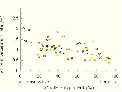
Figure 1. The percentage of white adult males incarcerated in each state vs. the state's average LQ. High white incarceration rates are found mostly in conservative states, low rates mostly in liberal states. The relationship is strong and linear. The regression line is shown dashed. (R = -0.56.)
We seek a measure of a state's conservative leanings. Conservative-leaning states tend to incarcerate all groups at high rates. But we cannot use a state's incarceration rate to measure conservatism because the total rate is strongly dependent on racial and ethnic mix. State's with high proportions of blacks, for example, will have high incarceration rates simply because the black rate of incarceration is so high. A single-group incarceration rate does not suffer from this difficulty. It can work well to gauge conservatism. We chose the white incarceration rate as a proxy for conservative sentiment.Figure 2 illustrates the disparity paradox. The white incarceration rate is the independent variable. Notice that high disparity ratios are found mostly in progressive states, and low ratios mostly in conservative states. For adult males, the correlation between the disparity ratio and the white incarceration rate is strong and inverse (R = -0.54).
Aside from the strong inverse correlation between white incarceration and the disparity ratio, the most compelling feature of Figure 2 is the extraordinarily large disparity ratio found in the nation's capitol. The ultra-liberal, sixty-percent-black District of Columbia checks in off the charts with black male per capita incarceration 29.3 times that of whites.
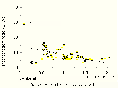
Figure 2. Black-to-white incarceration (disparity) ratios vary inversely with the white incarceration rate, a proxy for conservatism. R = -0.54. Relative to the regression line (shown dashed), the District of Columbia and Hawaii are prominent outliers.
Resolving the disparity paradox, wherein progressive states have the largest disparity ratios is the primary goal of this research. A secondary goal is to determine how criminality is distributed within white and black populations. The two goals are intertwined, because to resolve the paradox we need the distributions. When the dust settles, I suspect revealing some details of the criminality distributions will be the more important achievement. But let's get started.I begin with a quote from La Griffe du lion:
Sometimes human traits can be difficult to define, let alone measure. Still, we have a sense of their meaning. Take for example, "ambition." A man is not simply ambitious. He is very ambitious or moderately ambitious or not ambitious at all. Such properties vary by degree but resist precise quantitation. We call them fuzzy variables.
The pattern of behavior leading to arrest and imprisonment is, in the Griffian sense, a fuzzy variable. I call it criminality. To account for incarceration data, I propose the following three-part model.
1. Each racial group has its own characteristic, geography-invariant distribution of criminality.
2. Criminality distributions are approximately Gaussian (as mandated by the central limit theorem for properties resulting from many independent factors).
3. Political jurisdictions tolerate crime to varying degrees. They set thresholds of criminality, which when crossed result in incarceration. Thresholds differ by jurisdiction according to regional custom.
Figure 3 shows normalized distributions of criminality for black and white adult males. The distributions are Gaussian in accordance with the postulates. They have been rendered accurately in the figure by using parameter values obtained from the best least squares fit of calculated to observed disparity ratios. (See Appendix I for details.) The white criminality distribution lags behind the black. It is also broader. That is, whites display more variability. The black-white mean difference is 1.32 SD (in units of the white standard deviation); the (black/white) variance ratio is 0.76.
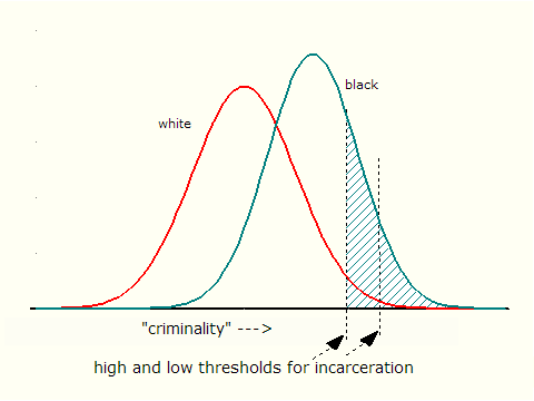
Figure 3. Distributions of criminality for adult black and white males. Thresholds for incarceration are shown for two states. They differ according to regional practice. The areas under the distribution curves to the right of the thresholds are the incarcerated fractions of the corresponding groups.
Two behavioral thresholds are shown in Figure 3. They correspond to different standards for incarceration applied in two different states. The lower threshold could have been set by a tough-on-crime, no-nonsense, conservative state like Oklahoma. In Oklahoma, it doesn't take much to land behind bars. The upper threshold belongs to a state with a higher tolerance for criminal behavior, say, New York. In each case, the incarcerated fraction of a group equals the area under its distribution curve to the right of the threshold. The ratio of these areas, black over white, is the disparity ratio. Figure 4 isolates these areas for the thresholds shown. High-threshold New York has the greater disparity ratio. If Figure 4 fails to convince you that moving an incarceration threshold to a higher level of criminality increases the disparity ratio, I present a more formal treatment in Appendix I.
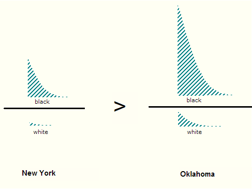
Figure 4. The ratio of areas representing the disparity ratio is shown schematically for two states. The ratio is greater in the more permissive, high-threshold New York than in the tough-on-crime, low-threshold Oklahoma.
Theory and observation
In Appendix I a relation between the incarceration ratio and the white incarceration rate is developed from our model. Figure 5 shows three of a family of curves illustrating the relation. The curves differ in the choice of parameter values in the criminality distributions. In the neighborhood of very small white incarceration (i.e., in ultra-liberal jurisdictions) the curves can be very steep, in part accounting for the extraordinary disparity ratio found in the District of Columbia.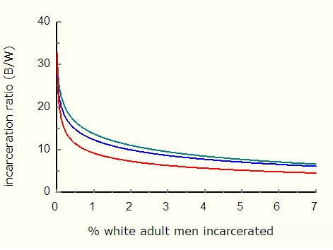
Figure 5. A family of curves relating the disparity ratio to white incarceration rates. The curves shown were generated by choosing different sets of parameter values in the criminality distributions.
We can determine the criminality distributions in the populations of adult black and white males by finding the curve in the family that, in the least squares sense, best fits observed incarceration data. However, any assessment of group criminality should include former as well as present felons. The incarceration data we have includes only those currently incarcerated.The number of living ex-prisoners is actually much greater than the number incarcerated. In 2001, for example, former prisoners accounted for 77% of all adult U.S. residents who had ever been incarcerated. Excluding them would seriously distort the analysis. As a zeroth order approximation, we estimated the number of men who were ever incarcerated by multiplying the inmate count by 77/23, the factor that would apply exactly if the 2001 figure applied across the board.
Figure 6 shows the best least-squares fit of incarceration ratio to the ever-incarcerated estimates. The predicted incarceration ratio cuts through the core of state data. It swings wildly upward when approaching super-liberal territory taking aim at the extreme incarceration ratio found in DC.
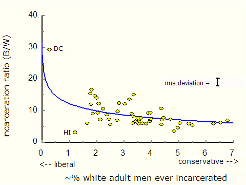
Figure 6. Variation of the disparity ratio with the percentage of white men ever incarcerated in fifty states and the District of Columbia. The predicted variation is shown by the curve.
In sum, we see that: 1) incarceration rates by state correlate strongly and inversely with the ADA "liberal quotient"; 2) variation of disparity ratios by state is well described by a model in which racial groups have characteristic, geography-invariant, Gaussian distributions of criminality; 3) applied to incarceration data, the model yields criminality distributions for adult black and white males, finding the black distribution narrower (variance ratio = 0.76), and displaced toward higher criminality values by 1.32 SD; the model predicts the disparity paradox, showing it to be an unintended result of setting high incarceration thresholds.
Thank you.
< polite applause >
I see Uncle Steve has signaled that we have time for a few questions. Yes ma'am?
First Professor: Are you saying that liberals are the cause of the disparity ratio?
Prodigy : No. The disparity ratio is greater than unity because blacks commit more crime per capita than whites. Liberals simply tweak the ratios upward by setting high incarceration thresholds in jurisdictions they control. The tweaking is sufficient to produce an observable trend in which the largest disparity ratios are found in progressive states. Isn't it ironic that the high disparity ratios found in progressive states are the result of the tolerance and goodwill we've learned to associate with progressive government?
Second Professor: The American Anthropological Association in its statement on race declares:
"The 'racial' worldview was invented to assign some groups to perpetual low status, while others were permitted access to privilege, power, and wealth. The tragedy in the United States has been that the policies and practices stemming from this worldview succeeded all too well in constructing unequal populations among Europeans, Native Americans, and peoples of African descent."
How does this square with your analysis?
Prodigy: I have simply described one consequence of the policies and practices stemming from the 'racial' worldview. As such, I hope anthropologists will welcome my findings. Sociologists too!
Third Professor: I notice in Figure 6 there is considerable scatter of the observed disparity ratios about the curve of predicted ratios. Why is that?
Prodigy: The curve in Figure 6 describes how disparity ratios would vary with white incarceration rates if the world were constructed exactly like my model. But the mapping of the model onto the real world is not perfect. Also, it would help if the estimates of ever-incarcerated percentages were replaced with actual observations. Nevertheless, the substantial agreement we do achieve indicates that the model incorporates the most salient features of the real world that bear upon the problem.
Fourth Professor: Can your analysis teach us how to reduce the disparity ratio?
Prodigy: It can, but you probably won't like what it tells us. I think we could all agree that the very best way to reduce the disparity would be by modifying the criminality distributions so that blacks and whites would commit crime at the same rate. But criminality distributions have stubbornly resisted change, leaving us only the incarceration thresholds to play with. To lower the disparity ratio in your state, simply lower the incarceration threshold imprisoning more bad guys of all stripes. That is the price you will have to pay to reduce the disparity ratio.
Sixth Professor: At the January Conference of the Society for Personality and Social Psychology, several presenters found correlations between political philosophy and racial bias. One study found that conservatives had stronger self-admitted and implicit biases against blacks than liberals did. Do you care to comment?
Prodigy: It does not surprise me. Of course, some might say that one man's bias is another's perspicacity.
Uncle Steve: Ahem. We can continue this over dinner. Thank you, Prodigy, for a stimulating talk, and for a refreshingly novel approach to a sociological problem undertaken honestly and with nobility of purpose. Speaking for sociologists, we do appreciate your explanation of a sociological bibelot that has puzzled us for years.
< enthusiastic applause >
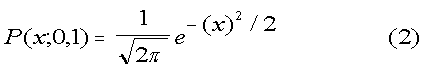
Both black and white criminality distributions are assumed Gaussian. That is, their distributions looks like this:
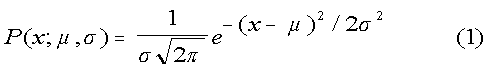
where μ and σ are the mean and standard deviation, respectively.
A simplification can be obtained by choosing the unit of criminality to be one standard deviation of the white distribution. Also, because we are interested only in the relative positions of the black and white distributions on the criminality axis, we can and do set the mean white criminality μW = 0. The white criminality distribution then looks like:
and the black distribution like:
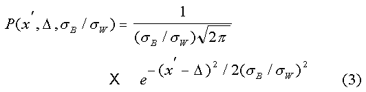
in which Δ is the mean difference, μB - μW. The primes are included to remind us that we used the transformations, x' = x / σW and dx' = dx / σW to arrive at (3). Note that with our choice of units, the black distribution depends on the dimensionless ratio of standard deviations, σB / σW.
The dependence of the disparity ratio on the white incarceration rate, plotted in Figure 6, is obtained as follows. The fraction of white-adult males ever imprisoned is given by:
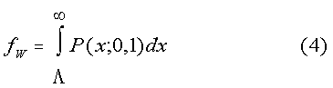
where Λ is the criminality threshold measured from the zero of the white distribution. The inverse function, Λ(fW), is obtained numerically. The ever-incarcerated fraction of blacks, given by
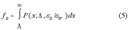
may then be evaluated for particular values of Δ and σB / σW , and the disparity ratio, fB / fW , computed.
The quantities, Δ and (σB / σW) were adjusted to give the best least squares fit of the calculated disparity ratios, fB / fW , to the observed ratios.
|
non-Hispanic White |
Black |
Ratio B/W |
||||
|
Alabama |
1.055 |
6.084 |
5.77 |
|||
|
Alaska |
0.745 |
4.233 |
5.68 |
|||
|
Arizona |
1.607 |
9.478 |
5.90 |
|||
|
Arkansas |
1.307 |
7.428 |
5.68 |
|||
|
California |
1.312 |
9.304 |
7.09 |
|||
|
Colorado |
1.161 |
10.729 |
9.24 |
|||
|
Connecticut |
0.542 |
8.985 |
16.58 |
|||
|
Delaware |
1.046 |
8.05 |
7.70 |
|||
|
D. C. |
0.083 |
2.432 |
29.30 |
|||
|
Florida |
1.503 |
9.117 |
6.07 |
|||
|
Georgia |
1.485 |
6.775 |
4.56 |
|||
|
Hawaii |
0.363 |
1.12 |
3.09 |
|||
|
Idaho |
1.441 |
5.085 |
3.53 |
|||
|
Illinois |
0.621 |
7.575 |
12.20 |
|||
|
Indiana |
1.083 |
8.288 |
7.65 |
|||
|
Iowa |
0.905 |
10.987 |
12.14 |
|||
|
Kansas |
1.184 |
11.036 |
9.32 |
|||
|
Kentucky |
1.328 |
10.343 |
7.79 |
|||
|
Louisiana |
1.187 |
8.415 |
7.09 |
|||
|
Maine |
0.636 |
4.547 |
7.15 |
|||
|
Maryland |
0.82 |
5.649 |
6.89 |
|||
|
Massachusetts |
0.61 |
5.682 |
9.31 |
|||
|
Michigan |
1.043 |
7.596 |
7.28 |
|||
|
Minnesota |
0.578 |
8.459 |
14.63 |
|||
|
Mississippi |
0.993 |
6.01 |
6.05 |
|||
|
Missouri |
1.178 |
7.739 |
6.57 |
|||
|
Montana |
1.022 |
6.72 |
6.58 |
|||
|
Nebraska |
0.669 |
7.067 |
10.56 |
|||
|
Nevada |
1.646 |
8.907 |
5.41 |
|||
|
New Hampshire |
0.71 |
6.164 |
8.68 |
|||
|
New Jersey |
0.528 |
8.104 |
15.35 |
|||
|
New Mexico |
0.828 |
8.085 |
9.76 |
|||
|
New York |
0.534 |
6.377 |
11.94 |
|||
|
North Carolina |
0.732 |
5.297 |
7.24 |
|||
|
North Dakota |
0.494 |
2.939 |
5.95 |
|||
|
Ohio |
0.981 |
8.857 |
9.03 |
|||
|
Oklahoma |
1.951 |
12.164 |
6.23 |
|||
|
Oregon |
1.404 |
10.119 |
7.21 |
|||
|
Pennsylvania |
0.845 |
10.482 |
12.40 |
|||
|
Rhode Island |
0.598 |
8.392 |
14.03 |
|||
|
South Carolina |
1.095 |
6.578 |
6.01 |
|||
|
South Dakota |
1.303 |
13.919 |
10.68 |
|||
|
Tennessee |
1.138 |
6.712 |
5.90 |
|||
|
Texas |
1.873 |
11.036 |
5.89 |
|||
|
Utah |
1.003 |
8.061 |
8.04 |
|||
|
Vermont |
0.555 |
5.026 |
9.06 |
|||
|
Virginia |
1.194 |
8.707 |
7.29 |
|||
|
Washington |
1.073 |
6.929 |
6.46 |
|||
|
West Virginia |
1.004 |
15.154 |
15.09 |
|||
|
Wisconsin |
0.955 |
12.993 |
13.61 |
|||
|
Wyoming |
2.028 |
14.037 |
6.92 |
|||
|
National |
1.072 |
7.923 |
7.39 |
|||
|
|
||||||
|
*Based on 2000 census data collected by Human Rights Watch |
||||||